Overview
This project aimed to explore path planning algorithms in continuous and discrete space. The following global path planning algorithms implemented are D* Lite, Theta*, and Potential Fields.
All algorithms were implemented in C++ as ROS packages from scratch. The planning and control framework is part of a larger ROS navgiation stack for autonomous driving using a TurtleBot.
The content for this project was developed by myself and three colleagues at Northwestern University. You can view the lectures for more information.
See the code in my GitHub repository.
Path Planning
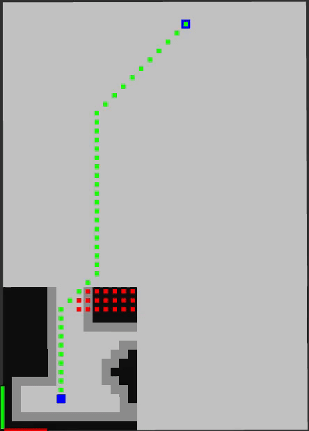
D* Lite
The implementation contains two internal representations of the grid map as 2D occupancy grids. The first is the complete map with all the obstacles. The second map is initialized empty and obstacles are added based on the visibility range of the robot.
This algorithm plans from the goal to the starting location. Originally, the shortest path is a straight line to the goal. As the path front moves toward the goal, obstacles come into view, the map updates, and the algorithm replans. The heuristic used here is euclidean distance.
The green cells represent the current shortest path. The red squares are the cells that are updated during the replanning stage after the map update. Below, the algorithm has a visibility horizon of 8 cells.
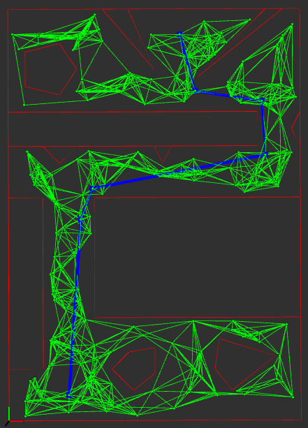
Theta*
A probabilistic roadmap is constructed by sampling points randomly in free space and connecting them to their nearest neighbors. Theta* is similar to A; the only difference is Theta optimizes the shortest path by skipping over nodes that can be connected by a straight line.
The roadmap shown in green was constructed using 200 nodes where each node is connected to 10 of its nearest neighbors. The shortest path is shown in blue. The heuristic used is euclidean distance.
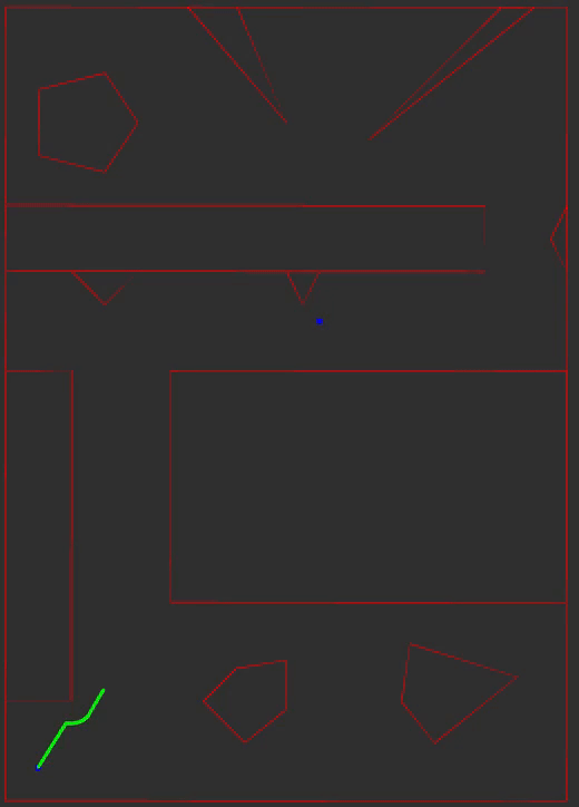
Potential Fields
An attractive gradient pulls the path front to the goal and a repulsive gradient repels the path front away from obstacles. The next position in the path front is obtained using one step of gradient descent. The descent direction is composed by summating the attractive and repulsive gradients and normalizing the sum using the L2-norm.
The green line is the path, the blue dots are the start/goal positions, and the red lines are the obstacle edges and bounds of the map.