Overview
The goal of this project was to implement Rao-Blackwellized Particle Filter SLAM from scratch. This is also known as FastSLAM for grid mapping or gmapping in the ROS community. See the code in my GitHub repository.
Results
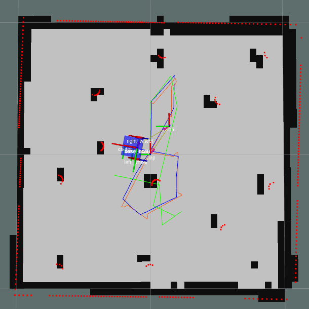
The ground truth path from gazebo is orange, SLAM is blue, and odometry is green. The final error in the pose relative to gazebo is given below. The map was created using 40 particles.
The odometry drifts further from the ground truth the longer the trajectory.
| X Error (cm) | Y Error (cm) | Yaw Error (degrees) | |
|---|---|---|---|
| Odometry | 19.5 | -10.5 | 2.62 |
| RBPF SLAM | -1.04 | 3.81 | 1.98 |
Rao-Blackwellized Particle Filters
Given the robot’s trajectory \(x_{1:t} = x_1,...,x_t\), the observations \(z_{1:t} = z_1,...,z_t\), and the odometry measurements \(u_{1:t-1} = u_1,...,u_{t-1}\) an estimate of the joint posterior \(p(x_{1:t}, m \mid z_{1:t}, u_{1:t-1})\) about the map, m, is computed [1]. The filter relies on the factorization below.
\[\begin{equation} p(x_{1:t}, m \mid z_{1:t}, u_{1:t-1}) = p(m \mid x_{1:t}, z_{1:t}) · p(x_{1:t} | z_{1:t}, u_{1:t−1}) \end{equation}\]The factorization allows us to first approximate the trajectory and then compose the map given the trajectory. This technique is referred to as Rao-Blackwellization. The computations is efficient because map is strongly dependent on the robot’s pose.
Implementation
See the full implementation.
1. An initial guess \(x^{'(i)}_t = x^{(i)}_{t-1} \oplus u_{t-1}\) of the robot’s pose is composed using the compound operator for each particle, i. The operator \(\oplus\) is the change in odometry \(\delta{x_t} = x_t - x_{t-1}\).
2. Iterative closest point (ICP) is used to estimate the change in the robot’s pose from the previous pose estimate. The initial guess of the robot’s pose \(x^{'(i)}_t\) is used as the starting point for ICP. If ICP fails, steps 3 and 4 are ignored. The pose of each particle \(x^{(i)}_t \sim p(x^{'(i)}_t \mid u_{t-1})\) is sampled using a probabilistic motion model. The weights are updated \(w^{(i)}_t = w^{(i)}_{t-1} \cdot p(z_t \mid m^{(i)}_{t-1}, x^{(i)}_t)\) using the scan likelihood model presented in Probabilistic Robotics Table 6.3.
3. A set of samples are drawn around \(\hat{x}^{(i)}_t\) reported by ICP. The mean and covariance of the proposal are updated by evaluating the target distribution \(p(z_t \mid m^{(i)}_{t-1}, x_j) \cdot p(x_j \mid x^{(i)}_{t-1}, u_{t-1})\) for each sampled pose $x_j$.
4. The new pose of each particle is drawn from the proposal distribution \(x^{(i)}_t \sim \mathcal{N}(\mu^{(i)}_t,\Sigma^{(i)}_t)\).
5. Update the importance weights.
6. Update the map \(m^{(i)}\) for each particle \(x^{(i)}_t\) given the observation \(z_t\).
7. The number of effective particles is updated \(N_{eff} = \frac{1}{\sum_{n=1}^{N} (\hat{w}^{(i)})^2}\), where \(\hat{w}^{(i)}\) is the normalized weight of each particle. If \(N_{eff} < N / 2\) ,where \(N\) is the number of particles, low variance resampling is used to replace the particles.
Algorithms Implemented
- The Rao-Blackwellized Particle Filter Algorithm presented in [1].
- Iterative Closest Point - Point Cloud Library ICP solver
- Occupancy Grid Mapping - Probabilistic Robotics Table 9.1
- Updated the Occupancy Grid using Raycasting Bresenham’s line algorithm
- Pose Likelihood - Probabilistic Robotics Table 5.5
- Scan Likelihood - Probabilistic Robotics Table 6.3
Credits
[1] Grisetti, Giorgio, Cyrill Stachniss, and Wolfram Burgard. “Improved techniques for grid mapping with rao-blackwellized particle filters.” IEEE transactions on Robotics 23.1 (2007): 34-46. PDF