Overview
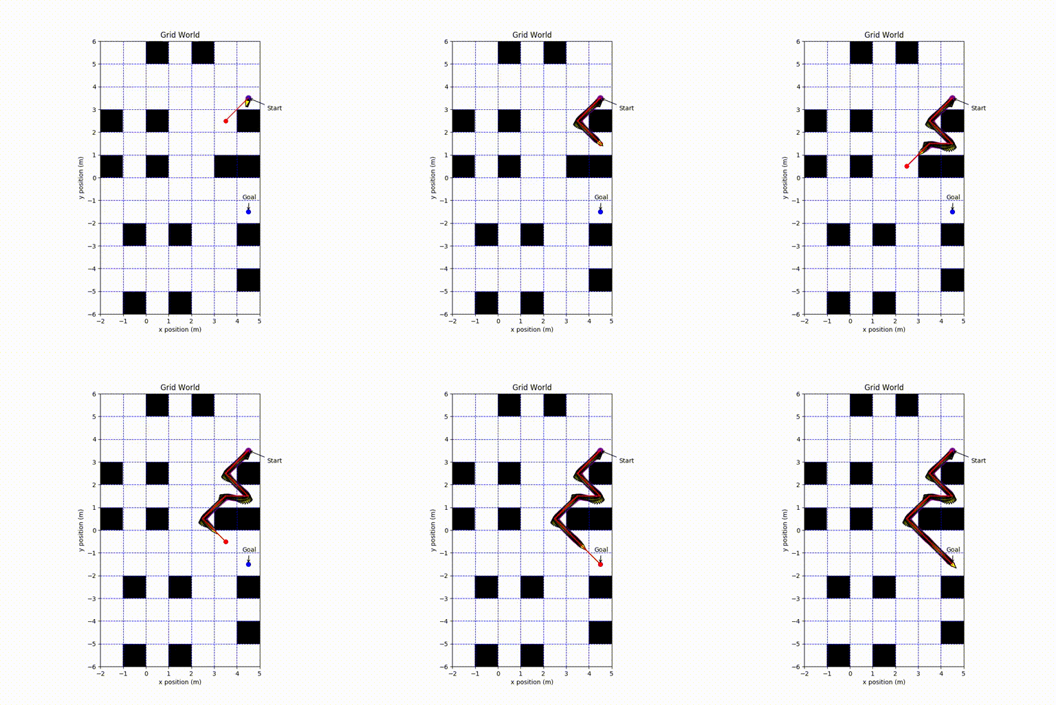
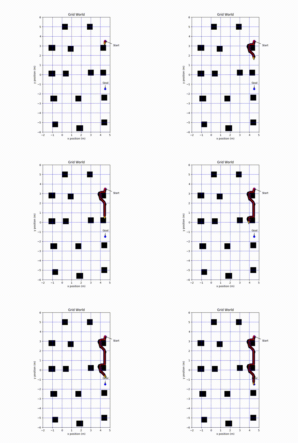
The project focus was to develop an online implementation of A* that does not have knowledge of the obstacles a priori and must re-plan from the current node when an obstacle is encountered. Additionally, the robot drives the path while planning from its current location using an inverse kinematic controller. If the robot ends up in a cell other than the target cell, A* must select a new target cell. The robot’s kinematics and noise added in the controller influence the path planning component by simulating stochasticity in the environment. All visualizations use the following color scheme: the start/end configurations are blue, the planned path using A* is red, the position of the robot is purple, the heading of the robot is depicted by a yellow arrow, all obstacles are black, and all unoccupied cells are white. See the code in my GitHub repository.
The grid discretizations below are 1m (left) and 0.1m (right).


Implementation
Heuristic
The implementation of A* use the Octile distance heuristic. On a square grid, the heuristic considers eight directions of movement. Given the position of the current node \((x_n, y_n)\) and the goal \((x_g, y_g)\), the heuristic is calculated as follows.
\[\begin{equation} h(n) = D_1 \, (dx + dy) + (D_2 - 2 \, D_1) \, min(dx, dy) \end{equation}\]The absolute differences in the horizontal \(dx\) and vertical \(dy\) positions are between the node and the goal, \(dx = \mid x_n - x_g \mid\) and \(dy = \mid y_n - y_g \mid\), \(D_1\) is the distance to an unoccupied node (north, south, east, or west), and \(D_2\) is the diagonal distance to an unoccupied node (\(D_1 =1\) and \(D_2 = \sqrt{2}\)). Let \(\gamma = D_2 - 2 \, D_1\) and the true cost \(\Lambda = D1 \, (dx + dy)\), if \(\gamma < 0\) the heuristic will not over-estimate the true cost because \(\Lambda\) will be reduced by \(\gamma \, min(dx, dy)\) therefore, the Octile distance heuristic is admissible.
Algorithm
The online algorithm determines the costs of all the neighboring nodes up to eight neighbors. If a neighboring node is already on the closed list, the neighboring node is ignored. The neighboring node with the smallest total cost is selected and placed on the open list. The open list will only have one node at a time in contrast to the naive implementation that will likely have an open list with more than one node.
The function below contains the implementation of A* online. It relies on a priority queue (not required for the online algorithm but improves efficiency) to determine the node with the minimum cost.
def online(self):
    """ A* online creates path from start to goal and
    only places lowest cost neighbor on openlist
    """

    while self.open_list:

        min_node = heapq.heappop(self.open_list)
        self.curr_node = min_node

        if self.curr_node.position == self.goal:
            print("Goal Reached by A* Planner")
            break

        self.closed_list.append(min_node)

        # determine neighboring cells and
        # compute cost of neighboring cells
        self.neighbor_cells_online()
First, create a class to store relevant data for each node.
class Node(object):
    """ creates a node for Astar """

    def __init__(self, parent, position):
        # costs for node
        self.g = 0      # true cost
        self.h = 0      # heuristic cost
        self.f = 0      # total cost

        # parent nodes and position of node
        self.parent = parent
        self.position = position

    def __lt__(self, other):
      # method fo comparisson for heapq
      return self.f < other.f
Next, find the neighboring node with the smallest cost and place on the open list. The actions must not direct the path off the grid. If the new node is already on the closed list at the same position, the new node is not added.
def neighbor_cells_online(self):
    """ determines neighboring cells for online algorithm """

    # clear all neighbors each time
    self.neighbors.clear()

    # current indices in grid world
    curr_x = self.curr_node.position[0]
    curr_y = self.curr_node.position[1]

    # evaluate neighbors
    for act in self.actions:
        # neighbors position
        temp_pos = [curr_x + act[0], curr_y + act[1]]

        # within bounds of grid world and not on lists
        if self.neighbor_bounds(temp_pos):
            continue


        # cost of potential new node
        new_node = self.neighbor_cost(temp_pos)

        # if on closed list ignore new node
        if new_node.position in [node.position for node in self.closed_list]:
            continue

        # append all neighbors for evaluation
        self.neighbors.append(new_node)


    # select neighbor with lowest cost
    best_neighbor = self.neighbors[0]
    for index, neighbor in enumerate(self.neighbors):
        if neighbor.f < best_neighbor.f:
            best_neighbor = neighbor

    # place lowest cost neighbor on openlist
    heapq.heappush(self.open_list, best_neighbor)
This function creates a new node and computes the cost.
def neighbor_cost(self, cell):
    """ compute costs of a neighboring cell """

    # create new node
    parent = self.curr_node
    position = cell
    node = Node(parent, cell)

    # compute cost
    # check if grid contains obstacle were the neighbor is
    true_cost = self.curr_node.g + self.grid.world[cell[0]][cell[1]]

    heuristic_cost = self.heuristic(cell)

    node.g = true_cost
    node.h = heuristic_cost
    node.f = true_cost + heuristic_cost

    return node
Inverse Kinematic Controller
The inverse kinematic controller models the robot as a kinematic unicycle, where \(u_1\) and \(u_2\) are the linear and angular velocity control inputs. In the frame of the robot the positive x-direction is forward and the positive y-direction is left. Positive angular velocity and angular position is considered counter clockwise. The kinematics are propagated forward using a fourth order Runge-Kutta integrator with a time step \(dt = 0.1s\).
\[\begin{equation} \begin{bmatrix} \dot{x}\\ \dot{y}\\ \dot{\theta} \end{bmatrix} = \begin{bmatrix} u_{1}cos(\theta)\\ u_{1}sin(\theta)\\ u_{2} \end{bmatrix} \end{equation}\]Given the pose of the robot (\(x, y, \theta\)) and a target position (\(x_T\), \(y_T\)), the nominal controls \(u_1\) and \(u_2\) are determined using the distance to the target and the error in the robot’s heading towards the target. Both controls are issued at the same time allowing the robot to turn and move towards the target simultaneously.
\[\begin{equation} u_1 = k_1 \sqrt{(x_T - x)^2 + (y_T - y)^2} + \varepsilon_v \end{equation}\] \[\begin{equation} u_2 = k_2(\arctan2(\frac{y_T - y}{x_T - x}) - \theta) + \varepsilon_\alpha \end{equation}\]Where \(k_1\) and \(k_2\) are the feedback gains, \(\varepsilon_v\) and \(\varepsilon_\alpha\) are random perturbations in the nominal control inputs. The robot’s pose is now probabilistic because of the random perturbations. The random perturbations are drawn from normal Gaussian distributions with means equal to zero, \(\varepsilon_v \sim \mathcal{N}(0,\,\sigma_v^{2})\,\) and \(\varepsilon_\alpha \sim \mathcal{N}(0,\,\sigma_\alpha^{2})\,\). The controller uses the following parameters (\(k_1 = 0.5\), \(k_2 = 2\), \(\sigma_v = 0.01\), \(\sigma_\alpha = 0.0875\)).
The values for the parameters \(\sigma_v\) and \(\sigma_\alpha\) assume the robot’s linear and angular velocity can be modulated within a standard deviation of \(1 \, \frac{cm}{s}\) and \(0.0875 \, \frac{rad}{s} \approx5 \,deg\).
The values for the feedback gains were determined experimentally. If the gains are too high, the robot will over shoot the desired target and if they are too low, it will take a longer time to reach the target cell. The gain \(k_2\) must be greater than \(k_1\). If the robot’s linear velocity is too high, the robot will have difficulty turning towards the target. Initially, the gains were set low and then incrementally increased until many oscillations in the robot’s pose were observed. The gains were then slowly decreased until the oscillations decreased and the robot could achieve the target cell.
The robot has the following acceleration limits \(\dot{v}_{max} = 0.228 \, \frac{m}{s^2}\) and \(\dot{\omega}_{max} = 5.579 \, \frac{rad}{s}\). To ensure the robot does not exceed the acceleration limits, the nominal controls calculated are not issued yet. Based on the kinematics, the linear velocity of the robot is the control \(u_1\) and the angular velocity is the the control \(u_2\). The linear and angular accelerations of the robot are then computed using forward finite differences.
\[\begin{equation} a_l = \frac{u_{1_t} - u_{1_{t-1}}}{dt} \end{equation}\] \[\begin{equation} a_\alpha = \frac{u_{2_t} - u_{2_{t-1}}}{dt} \end{equation}\]Where \(a_l\) and \(a_\alpha\) are the tangential and angular accelerations, the robot will experience these accelerations if the nominal controls are issued. The variables \(u_{1_t}\) and \(u_{2_t}\) are the current nominal linear and angular controls, \(u_{1_{t-1}}\) and \(u_{2_{t-1}}\) were the controls issued at the previous time step. If the accelerations are greater than the acceleration limits, the controls issued are given below.
\[\begin{equation} u_1 = u_{1_{t-1}} + \dot{v}_{max} \, dt \end{equation}\] \[\begin{equation} u_2 = u_{2_{t-1}} + \dot{\omega}_{max} \, dt \end{equation}\]The control update ensures the acceleration limits are not exceeded because the max accelerations are considered during the update. The direction of acceleration needs to be considered. If an acceleration is negative, the corresponding limit used either \(\dot{v}_{max}\) or \(\dot{\omega}_{max}\) should be negative. Random perturbations are not applied here because there is no guarantee that the acceleration limits will not be exceeded.
The robot always starts with the speeds (\(v = 0 \, \frac{m}{s} and \omega = 0 \, \frac{rad}{s}\)) at the position of the start with a heading of \(\theta = \frac{-pi}{2}\). At each pose update from the Runge-Kutta integrator, noise was added to each of the states.
\[\begin{align*} x_t &= x_t + \varepsilon_x, \qquad \varepsilon_x \sim \mathcal{N}(0,\,\sigma_x^{2}) \\ y_t &= y_t + \varepsilon_y, \qquad \varepsilon_y \sim \mathcal{N}(0,\,\sigma_y^{2}) \\ \theta_t &= \theta_t + \varepsilon_{\theta}, \qquad \varepsilon_{\theta} \sim \mathcal{N}(0,\,\sigma_\theta^{2}) \end{align*}\]The noise was drawn from a normal distribution with a mean of zero and the following standard deviations (\(\sigma_x = 0.02\), \(\sigma_y = 0.02\), and \(\sigma_{\theta} = 0.0875\)). The standard deviations for x and y positions correspond to \(2\,cm\) and the standard deviation for angular position is \(\approx 5\,deg\). The values are realistic for the motion model because smaller values are unlikely to capture stochasticity in the environment.